
James Fox, Cyber Security Operations Consultant | 29 February 2024
A common issue for threat hunters is forming a systematic approach to handle noisy hunt/detection results (without simply ignoring them of course). Importantly, we are going to define "noisy" here as containing a high number of benign positive results, rather than out-right false-positives which call into question the accuracy of the analysis itself. As such, we can name resultant events from "noisy" detections as weak indicators of malicious activity.
Unfortunately, weak indicators lead to weak or uncertain threat hunt results. But sometimes they can be the only reliable method for detecting that specific technique. This is particularly evident when hunting for evidence of techniques early in the kill-chain such as initial access. This can be helped through chaining threat hunting results into a cohesive attack narrative, thereby strengthening the uncertain determination by modelling relationships between weak indicators.
As an example, consider the following two events of interest.
Figure 1: Event showing a SharePoint document download anomaly
Figure 2: Event showing a sign-in from a new location
Withstanding justifying business context, these events in isolations are difficult to determine if they are the result of a malicious, or simply benign user activity. This is in part due to:
However (as you may have already noticed), we can build out some correlations between these events to paint a picture of suspected data-theft:
James FoxBy far the most important (and trickiest) correlation of these is time. Without considering the order of the events and their distance in time, building a cohesive attack narrative is impossible. There are numerous strategies for building these correlations depending on the data and context of the event. We'll go through some of the more interesting ones by using examples to justify were they are most appropriately applied.
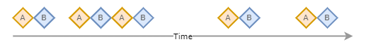
LNK files, or Windows shortcut files, are files which are designed to link to executable programs, files or folders. Malicious LNKs disguised as benign file types can be crafted by threat actors and delivered to unsuspecting users and have been exceedingly prevalent as a first-stage malware delivery mechanism.
When a user double-clicks on an LNK file two events are created by Microsoft Defender for Endpoint:
DeviceEvent with the action type BrowserLaunchedToOpenUrl. This event contains the full path to the LNK file in the RemoteUrl field.explorer.exe with the LNK target command line.Both the actual path to the LNK and the subsequent command line run are needed in a single result to determine if a LNK click is malicious - yet these events can't be joined together directly since they do not share a common field. It can't be assumed that the name or location of the LNK file relates in any way to it's target. However, there exists a strong temporal relationship between the events, notably that event A always results in a single instance of event B, and since event A and event B will always be close in time proximity event A and B will appear as ordered pairs.
Knowing this, the events can be combined simply by finding the nearest event B, given some event A in an ordered set of event A and B. We can do this very simply in Python using Pandas.
        import pandas as pd

        # Read the CSV files that contain our events into Pandas DataFrames
        df_event_a = pd.read_csv("example2-event-a.csv")
        df_event_b = pd.read_csv("example2-event-b.csv")

        # Convert the time fields to Pandas timestamps
        df_event_a["Timestamp_Firewall"] = pd.to_datetime(df_event_a["Timestamp_Firewall"])
        df_event_b["Timestamp_VPN"] = pd.to_datetime(df_event_b["Timestamp_VPN"])

        # Compute the cross product between the data frames using a dummy join key
        df_event_a['key'] = 0
        df_event_b['key'] = 0

        crossp_events = pd.merge(df_event_a, df_event_b, on='key').drop('key', axis=1)

        # Filter out where the difference in timestamps is less than our buffer
        buffer = pd.Timedelta(minutes=2)
        merged_events = crossp_events[
            (crossp_events['Timestamp_VPN'] >= crossp_events['Timestamp_Firewall']) &
            (crossp_events['Timestamp_VPN'] - crossp_events['Timestamp_Firewall'] <= buffer)
        ]
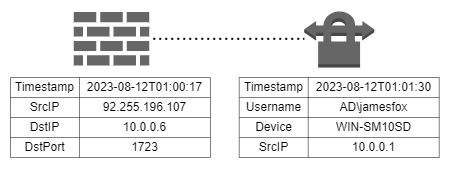
In this example, we are going to consider hunting for VPN connections from suspicious source IP addresses or locations, which may indicate that a threat actor has breached the internal network through valid VPN credentials. The pieces of information that we need to build a valuable detection would be:
To make things interesting, the log data supplied by the VPN server is limited. In the case of a successful VPN connection the VPN server will create an entry in the Application Event Log (Event A) that contains the authenticating username and the name of the device connecting. However, this VPN server is behind a firewall, so the source IP address of the connection is just the IP address of the firewall. The firewall logs all incoming accepted connections to the VPN server (Event B).
Unlike LNK click events, we can not simply match event A with the nearest event B. This is because:
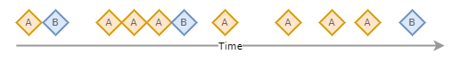
Even though for all event B there must exist some event A, there is uncertainty in which event A actually resulted in event B. We can model this uncertainty by using some domain knowledge to specify a maximum time buffer between event A and B, and then filter all event A for where there is a subsequent event B in the time buffer. In our VPN example, we would expect the time taken between the firewall log and the successful VPN connection to be within 2 minutes, as this is how long most users will take to type in their password.
We are going to use the Python Pandas library again, this time to cross-product the two event tables and filter where the difference between timestamps is less than our allowable buffer.
        import pandas as pd

        # Read the CSV files that contain our events into Pandas DataFrames
        df_event_a = pd.read_csv("example2-event-a.csv")
        df_event_b = pd.read_csv("example2-event-b.csv")

        # Convert the time fields to Pandas timestamps
        df_event_a["Timestamp_Firewall"] = pd.to_datetime(df_event_a["Timestamp_Firewall"])
        df_event_b["Timestamp_VPN"] = pd.to_datetime(df_event_b["Timestamp_VPN"])

        # Compute the cross product between the data frames using a dummy join key
        df_event_a['key'] = 0
        df_event_b['key'] = 0

        crossp_events = pd.merge(df_event_a, df_event_b, on='key').drop('key', axis=1)

        # Filter out where the difference in timestamps is less than our buffer
        buffer = pd.Timedelta(minutes=2)
        merged_events = crossp_events[
            (crossp_events['Timestamp_VPN'] >= crossp_events['Timestamp_Firewall']) &
            (crossp_events['Timestamp_VPN'] - crossp_events['Timestamp_Firewall'] <= buffer)
        ]
In some data sets this method may result in an excessive amount of results due to taking a cross product. In this case, consider determining the time buffer experimentally or by filtering the events for before computing the cross product (E.G removing VPN connections from devices which match an expected device naming scheme).
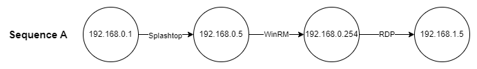
For our last example, we are going to hunt for evidence of nested remote desktop connections in a network. We are particularly interested in instances where remote desktop connections are chained together. For example, a user logs into host B from host A, then the user logs into host C from host B. This might be indicative of a threat actor moving throughout the network through a set of compromised credentials. To complicate matters, we are going to use only network logs to form this analysis - so we can't cheat by building out device sessions.
TimeGenerated
SrcIP
DestIP
PacketMatch
Figure 6: Example remote desktop network traffic logs
In all previous methods, we've built temporal correlations by sequencing two sets of events, but in this case we can't assume that only two events form a sequence. In fact, the more events that can be correlated together the more suspicious the activity becomes. We can instead approach this by creating a directed graph of the remote desktop connections, then traversing this graph using DFS with a time constraint to build up the sequences.
Again, we are going to use Python Pandas to achieve this. To take most of the effort away from building the graph data structure we are also going to use the Network X library too. Unfortunately, Network X doesn't provide a nice way to add constraints to DFS search so we will have to implement that separately in the function time_constrained_dfs.
        import networkx as nx
        import pandas as pd
        from datetime import datetime, timedelta

        def time_constrained_dfs(G, source, buffer):
            '''
            Run DFS on directed graph G from a source, based on a given time constraint.
            '''
            visited = set()
            stack = [(source, None, [source])]

            sequences = []

            while stack:
                node, parent_time, path = stack.pop()

                if node not in visited:
                    visited.add(node)

                    for _, next_node, key in G.out_edges(node, keys=True):
                        edge_data = G[node][next_node][key]
                        edge_time = edge_data["timestamp"]

                        if parent_time is None or (edge_time - parent_time) <= buffer:
                            new_path = path + [next_node]
                            sequences.append(new_path)
                            stack.append((next_node, edge_time, new_path))

            return sequences

        # Read our data into a Pandas dataframe
        df = pd.read_csv("example3-event-a.csv")

        # Create a multigraph. This is needed since each edge is representative of a timestamp and remote access method
        G = nx.MultiDiGraph()

        for index, row in df.iterrows():
            # String format the date-time into the expected date object needed
            timestamp = datetime.strptime(row['TimeGenerated'], '%Y-%m-%dT%H:%M:%S%z')
            # Add the edge to the graph
            G.add_edge(row['SrcIP'], row['DestIP'], timestamp=timestamp, packet=row['PacketMatch'])

        # Set the maximum time buffer to 2h
        buffer = timedelta(hours=2)

        # Get sequences from all nodes
        all_sequences = []
        for node in G.nodes():
            all_sequences.extend(time_constrained_dfs(G, node, buffer))

        # Filter out non-nested sequences
        nested_sequences = [seq for seq in all_sequences if len(seq) > 2]

        # Print the nested sequences
        for seq in nested_sequences:
            print(" -> ".join(seq))
Given the sample data above, the found sequences are:
        192.168.0.1 -> 192.168.0.5 -> 192.168.0.254
        192.168.0.1 -> 192.168.0.5 -> 192.168.0.254 -> 192.168.1.5
        192.168.0.5 -> 192.168.0.254 -> 192.168.1.5
Note that this code snippet is intended to return multiple sequences for those over size 2. For example the above sequence of size 4 starting from 192.168.0.1 can also begin from 192.168.0.5, and thus another sequence of size 3 is found . The most significant sequence is the superset of all found sequences (taking into account that sequence elements are distinct by time and method).
In this blog post we've gone through 3 different examples of how to build temporal correlations between data points in threat hunts. These are often necessary in order to form attack narratives from weak malicious indicators or to join data missing a unifying key. The following table outlines the pros and cons of each of the explored methods.
Request a consultation with one of our security specialists today or sign up to receive our monthly newsletter via email.
Get in touch Sign up!